A concise tutorial of neural networks
Neural networks are the fundamental model architectures of modern deep learning. This tutorial explains the basic mathematics in neural networks and its applications. A general neural network model is implemented from scratch with python.
1. Theory
1.1 Simple description
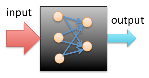
Consider a black-box with input and output, as shown below, a neural network is a "model" that "learns" the mechanism inside of this black-box, based on limited datasets of input and output.
1.2 Mathematic perspective
Neural network is a speific type of parameterized functions (mapping) \(f(\cdot): \mathbb{R}^{n_i} \to \mathbb{R}^{n_o}\) that is consisted by linear projections and 1D-activation functions.
Given limited number of samples of input (\(x^{(i)} \in X \subset \mathbb{R}^{n_i}\)) and output (\(y^{(i)} \in Y \subset \mathbb{R}^{n_o}\)), where \(i=1,2,...,m\) (m is the number of samples), the task of the NN algorithm is to optimize (learn) the parameters (weights) in the NN.
The following diagram shows a general framework of neural networks with L layers:
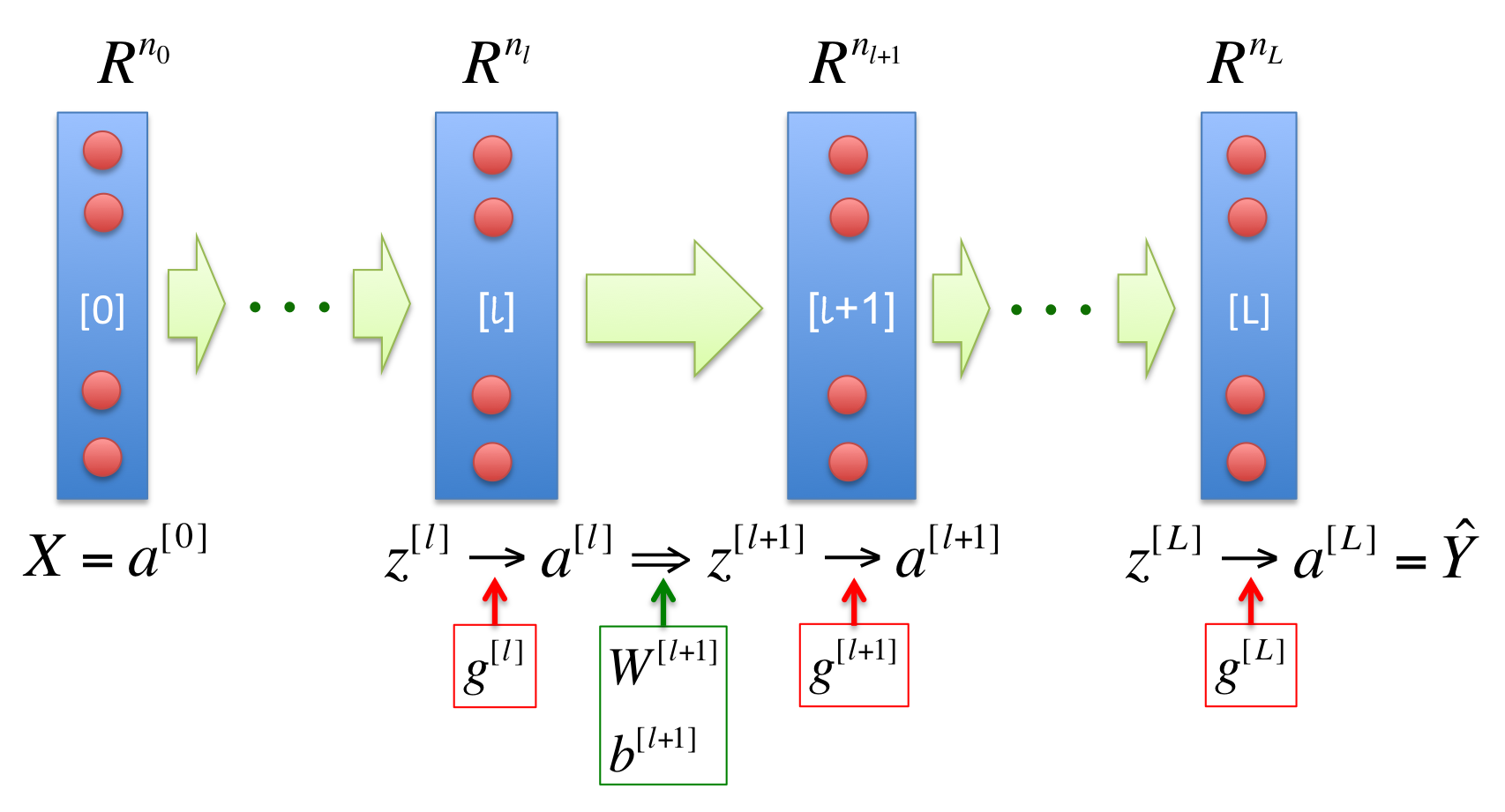
Where, the square brackets [] in the superscripts represent the layer; the green thick arrows represent the linear transformation, with W and b as the weights and biases, respectively; the red cycles represent the neurons, where 1D-activation functions \(g(z)\) works to project the variable \(z\) to activated variable \(a\); the number \(n_l\) on the top represents the dimension number of the \(l^{th}\) layer.
1.3 Core algorithm
The core calculations includes three steps: forward propagation, back propagation, and gradient descent optimization. The forward propagation moves from left to right, and finally gets the loss (cost) functions. The back propation calculates the errors from right to left, and finally gets the partial derivative of cost function to each parameter (W and b). Here, we take the calculation from the \([l]^{th}\) layer (\(a^{[l]}\)) to the \([l+1]^{th}\) layer (\(a^{[l+1]}\)) as an example:
a) Forward propagation
\(z^{[l+1]} = W^{[l+1]} a^{[l]} + b^{[l+1]}\)
\(a^{[l+1]} = g^{[l+1]}(z^{[l+1]})\)
b) Back propagation
\(\delta z^{[l+1]} = \delta a^{[l+1]} \circ g'(z^{[l+1]})\)
\(\delta W^{[l+1]} = \frac{1}{m} \delta z^{[l+1]} a^{[l]T} \)
\(\delta b^{[l+1]} = \frac{1}{m} \sum_{i=1}^m \delta z^{[l+1](i)} \)
\(\delta a^{[l]} = W^{[l+1]T} \delta z^{[l+1]}\)
c) Gradient descent
\(W := W - \alpha \delta W\)
\(b := b - \alpha \delta b\)
Where, \(\delta (\cdot)\) represents the partial derivative of the cost function \(\frac{\partial J(\hat{y},y)}{\partial (\cdot)}\) (or errors); \(\circ\) represents Hadamard product of two matrixes; the sizes of \(z^{[l]}, a^{[l]}, \delta z^{[l]}, \delta a^{[l]}\) are \((n_l, m)\); the sizes of \(z^{[l+1]}, a^{[l+1]}, \delta z^{[l]}, \delta a^{[l]}\) are \((n_{l+1}, m)\); the size of \(W^{[l+1]}\) is ; the size of \(b^{[l+1]}\) is \((n_{l+1}, 1)\); \(\alpha\) is the learning rate.
In practice, the back propagation is from \(\delta z^{[l+1]}\) to \(\delta z^{[l]}\), and the derivative of the activation function can be writen as a function of the activation function itself: \(g'(z) = G[g(z)]\). Therefore, we have the new form of the back propagation algorithm:
\(\delta W^{[l+1]} = \frac{1}{m} \delta z^{[l+1]} a^{[l]T}\)
\(\delta b^{[l+1]} = \frac{1}{m} \sum_{i=1}^m \delta z^{[l+1](i)} \)
\(\delta z^{[l]} = W^{[l+1]T} \delta z^{[l+1]} \circ G(a^{[l]})\)
Where, \(G(a^{[l]}) = g'(z^{[l]})\)
1.4 Compare with linear and logistic regression
If there is only one layer in the neural network (no hidden layer), the NN reduces into linear or logistic regression, depending on the activation function. If identity function \(g(x)=x\) is used for the activation function, the NN becomes a linear regression model. One-hidden layer NN could be used as Fourier transform if you specify the weights to the corresponding Fourier transform coefficients.
1.5 Model parameters
1.5.1 Activation functions
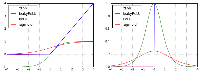
Activation functions are the only places that introduce nonlinearities into the NN. Here, we list several classic nonlinear activation functions:
a) Sigmoid function
\(g(z) = \frac {1} {1+e^{-z}}\)
\(g'(z) = \frac {e^z} {(e^z+1)^2} = g(z)[1-g(z)]\)
b) Tanh (hyperbolic) function
\(g(z) = \frac {e^z - e^{-z}} {e^z + e^{-z}}\)
\(g'(z) = \frac {4e^{2z}} {(e^{2z}+1)^2} = 1 - g^2(z)\)
c) ReLU (rectified linear unit) function
\(g(z) = max(0, z)\)
\(g'(z) = \left\{\begin{array}=z, if z>0 \\0, else\end{array}\right.\)
d) Leaky ReLU (rectified linear unit) function
\(g(z) = max(0.01z, z)\)
\(g'(z) = \left\{\begin{array}=1, if z>0 \\0.01, else\end{array}\right.\)
Empirically, the performance of these activation functions from better to worse is: ReLU ~ Leaky ReLU > Tanh > sigmoid.
import numpy as np

def factgrad(z, function='sigmoid'):
    if function == 'sigmoid':
        gz = 1.0/(1 + np.exp(-1.0*z) )
        return gz, gz*(1.0-gz)
    if function == 'tanh':
        gz = (np.exp(2.0*z) - 1) / (np.exp(2.0*z) + 1)
        return gz, 1.0-gz*gz
    if function == 'ReLU':
        gz = np.maximum(z*0, z)
        grad = z*0; grad[z>0] = 1.0
        return gz, grad
    if function == 'leakyReLU':
        gz = np.maximum(z*0.01, z)
        grad = z*0 + 0.01; grad[z>0] = 1.0
        return gz, grad

import matplotlib
%matplotlib inline
import matplotlib.pyplot as plt

x = np.linspace(-4,4,201)
gstrs = {'sigmoid':'r','tanh':'g','ReLU':'b','leakyReLU':'m' }

plt.figure(1, figsize=(12,4))
for k in [0, 1]:
    plt.subplot(1,2,k+1)
    for gstr in gstrs.keys():
        plt.plot(x, factgrad(x, function=gstr)[k], gstrs[gstr])
        plt.grid(True)
        plt.legend(gstrs.keys(), loc=2)
1.5.2 Loss and cost function
The loss function \(L(y^{(i)}, \hat{y}^{(i)}) = L(y^{(i)}, a^{[L](i)}) \) for one pair of samples \((x^{(i)}, y^{(i)})\), (i=1,2,...,m) can be defined as two types:
a) Cross-entropy loss function
\(L(y^{(i)}, \hat{y}^{(i)}) = \sum^{n_{L}}_{k=1} [-y^{(i)}_k ln(\hat{y}^{(i)}_k) - (1-y^{(i)}_k) ln(1 - \hat{y}^{(i)}_k) ]\)
b) Squared-error loss function
\(L(y^{(i)}, \hat{y}^{(i)}) = \frac{1}{2} \sum^{n_{L}}_{k=1} [y^{(i)}_k - \hat{y}^{(i)}_k]^2\)
The cost function is the summation of the loss functions for all samples:
\(J(Y, \hat{Y}) = \frac{1}{m} \sum^{m}_{i=1} L(y^{(i)}, \hat{y}^{(i)})\)
If the cross-entropy form is used for loss function and sigmoid function is used for activation function in the last layer ( layer), the calculation of the error in the last layer
can be simlified as:
\(\delta z^{[L]} = \delta a^{[L]} \circ g'(z^{[L]}) \\\ \ \ \ \ \ \ = \frac{\partial J}{\partial a^{[L]}} \circ G(a^{[L]}) \\\ \ \ \ \ \ \ = \frac{a^{[L]}-y}{a^{[L]}(1-a^{[L]})} \circ a^{[L]}(1-a^{[L]}) \\\ \ \ \ \ \ \ = a^{[L]} - y\)
1.5.3 Regularization
To prevent too large parameters and overfitting, regularization term is needed in the cost function:
\(J_{R}(Y, \hat{Y}) = J(Y, \hat{Y}) + \frac{\lambda}{2} \sum_{l=1}^{L} \parallel W^{[l]} \parallel ^ 2\)
Then, the partial derivatives of the cost function to the parameters become:
\(\delta_R W = \delta W + \lambda W\)
\(\delta_R b = \delta b\)
1.5.4 Learning rate
Learning rate \(\alpha\) is a tunable parameter. The large it is, the faster the learning speed is.
1.5.5 Feature generation
Additional features can be generated from known features by multiplication: \(x_1, x_2 \to x_1^2, x_2^2, x_1 x_2\)
1.5.6 Scaling
The input features should be normalized, otherwise the bias terms \(b\) will be too large.
1.5.7 Initialization
Initial weights (\(W\)) and biases (\(b\)) should be generated randomly to break down the "symmetry".
2. Applications
2.1 Implementation of NN from scratch with Python
class NN:
    def __init__(self, ndims=[1,1], activation=['sigmoid']):
        # weight: [(n[1], n[0]), ... ,(n[l+1], n[l]), ... ,(n[L], n[L-1])]
        # bias:   [(n[1],    1), ... ,(n[l+1],    1), ... ,(n[L],      1)]
        # activation: 'sigmoid', 'tanh', 'ReLU', 'leakyReLU'
        nlayer = len(ndims) - 1
        if len(activation) == 1:
            activation = activation * nlayer
        else:
            if len(activation) != nlayer:
                print 'ERROR: activation should have ', format(nlayer) ,' layers!'
                return
        self.nlayer = nlayer
        self.ndims  = ndims
        self.activation = activation
        self.weight = []
        self.bias   = []
        for i in range(self.nlayer):
            self.weight.append(np.random.rand(ndims[i+1], ndims[i]))
            self.bias.append(np.random.rand(ndims[i+1], 1))
        return

    def fpredict(self, x):
        # forward propagation
        a = [x]
        for i in range(self.nlayer):
            z = np.dot(self.weight[i], a[i]) + self.bias[i]
            tmp, ga = factgrad(z, function=self.activation[i])
            a.append(tmp)
        return a[1:]

    def flearning(self, x0, y0, scaling=True, loss='log', regu=0, lrate=0.03, niter=100):
        # --------------- input arguments -----------------
        # x0: (n[0], m)  input data
        # y0: (n[L], m)  output (labels)
        # scaling: x feature scaling
        # loss: 'log', 'square'
        # regu: 0 or positive value
        # lrate: learning rate
        # niter: maximum iteration number
        # ------------------- outputs ---------------------
        # costs: change of cost function (real number)
        # -------------------------------------------------

        m = x0.shape[1]
        # x features scaling
        if scaling:
            mx = np.sum(x0, axis=1, keepdims=True)/m
            sx = np.std(x0, axis=1, keepdims=True)
            x = (x0-mx) / sx
        else:
            x = x0

        # adjust the labels
        if self.activation[-1] == 'tanh':
            y = y0 + 0
            y[y==0] = -1
        else:
            y = y0

        # learning
        costs = []
        for i in range(niter):
            cost, dw, db = self.fcostgrad(x, y, loss=loss, regu=regu)
            costs.append(cost)
            for l in range(self.nlayer):
                self.weight[l] -= lrate*dw[l]
                self.bias[l] -= lrate*db[l]
        return costs

    def fcostgrad(self, x, y, loss='log', regu=0):
        # perform forward and back propagation;
        # calculate the cost function and the partial derivatives
        # --------------- input arguments -----------------
        # x: (n[0], m)
        # y: (n[L], m)
        # loss: 'log', 'square'
        # regu: 0 or positive value
        # ------------------- outputs ---------------------
        # cost: cost function (real number)
        # grad_w, grad_b: partial derivative of cost function to w, b
        #                 (the same size as weight and bias)
        # -------------------------------------------------

        m = x.shape[1]
        ndims = self.ndims[1:]
        z=[]; a=[x]; ga=[]; dz=[]; dw=[]; db=[]
        for i in range(self.nlayer):
            z.append(np.zeros([ndims[i], m]))
            a.append(np.zeros([ndims[i], m]))
            ga.append(np.zeros([ndims[i], m]))
            dz.append(np.zeros([ndims[i], m]))
            dw.append(self.weight[i]*0)
            db.append(self.bias[i]*0)

        # forward propagation
        for i in range(self.nlayer):
            z[i] = np.dot(self.weight[i], a[i]) + self.bias[i]
            a[i+1], ga[i] = factgrad(z[i], function=self.activation[i])

        # cost function
        if loss == 'log':
            cost = np.sum( -y*np.log(a[-1])-(1-y)*np.log(1-a[-1]) ) / m
            if self.activation[-1] == 'sigmoid':
                dz[-1] = a[-1] - y
            else:
                dz[-1] = (a[-1] - y)*ga[-1] /a[-1]/(1-a[-1])
        if loss == 'square':
            cost = 0.5*np.sum( (a[-1] - y)**2 ) / m
            dz[-1] = (a[-1] - y)*ga[-1]

        # add regularization to cost function
        if regu > 0:
            for i in range(self.nlayer):
                cost += 0.5*regu*np.sum(self.weight[i]**2)

        # back propagation
        for i in range(self.nlayer)[::-1]:
            dw[i] = np.dot(dz[i], a[i].T) + regu*self.weight[i] / m
            db[i] = np.sum(dz[i], axis=1, keepdims=True) / m
            if i>0:
                dz[i-1] = np.dot(self.weight[i].T, dz[i]) * ga[i-1]
        return cost, dw, db
Test case 1: four classes (linear)
def fxy2d(m=100, nclass=2, center=[[1,0], [0,1]]):
    ds = np.random.normal(0, 1.0, m)
    angs = np.random.rand(m)
    labels = np.random.rand(m)

    x = np.zeros([2, m])
    y = np.zeros([nclass, m])

    for i in range(nclass):
        index = (labels>=i*1.0/nclass) * (labels<(i+1)*1.0/nclass)
        x[0,index] = center[i][0] + ds[index]*np.cos(angs[index]*np.pi*2)
        x[1,index] = center[i][1] + ds[index]*np.sin(angs[index]*np.pi*2)
        y[i,index] = 1
    return x, y

nclass = 4
cstrs = ['ro','bo','go','mo','co','yo']
x,y = fxy2d(m=200, nclass=nclass, center=[[2,-2], [-2,2], [2,2], [-2,-2]])

for i in range(nclass):
    plt.plot(x[0, y[i,:]==1], x[1, y[i,:]==1], cstrs[i])

# NN learning
nnmodel = NN(ndims=[x.shape[0], 5, 4, y.shape[0]], activation=['sigmoid'])
costs = nnmodel.flearning(x, y, scaling=True, loss='log', regu=0, lrate=0.03, niter=200)

# prediction
npic = 21
xx,yy = np.meshgrid(np.linspace(-3,3,npic), np.linspace(-3,3,npic))
pr = nnmodel.fpredict(np.append( xx.reshape(1, npic**2), yy.reshape(1, npic**2), axis=0))

# plots
ncol = nnmodel.nlayer
nrow = np.max(nnmodel.ndims[1:])
plt.figure(1, figsize=(ncol*4, nrow*4))
for irow in range(nrow):
    for icol in range(ncol):
        if irow < nnmodel.ndims[icol+1]:
            plt.subplot(nrow,ncol,irow*ncol+icol+1)
            for i in range(nclass):
                plt.plot(x[0, y[i,:]==1], x[1, y[i,:]==1], cstrs[i])
            plt.contourf(xx,yy, pr[icol][irow,:].reshape(npic,npic), 20)
            #plt.colorbar()

plt.figure(2)
plt.plot(costs)
plt.title('cost function')
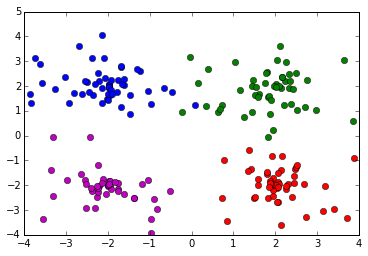
Distribution of data:
Activation function in the two hidden layers and output layer:
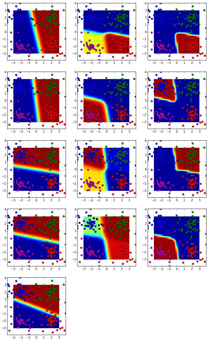
As shown here, the first hidden layer is indeed a linear classifier, and the following layers show more and more nonlinearity. This is the core of neural network: based on the approximation theory, any smooth non-linear function can be fitted by piecewise linear functions.
Loss function:
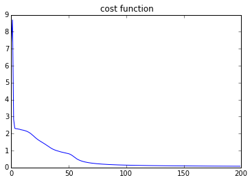
Test case 2: non-linear binary classification
def fxy2d_circle(m=100, nclass=2):
    ds = np.random.normal(0, 0.3, m)
    angs = np.random.rand(m)
    labels = np.random.rand(m)

    x = np.zeros([2, m])
    y = np.zeros([nclass, m])

    rs = [0, 2]
    for i in range(nclass):
        index = (labels>=i*1.0/nclass) * (labels<(i+1)*1.0/nclass)
        x[0,index] = (rs[i] + ds[index])*np.cos(angs[index]*np.pi*2)
        x[1,index] = (rs[i] + ds[index])*np.sin(angs[index]*np.pi*2)
        y[i,index] = 1
    return x, y

nclass = 2
cstrs = ['ro','bo','go','mo','co','yo']
x,y = fxy2d_circle(m=200, nclass=nclass)

for i in range(nclass):
    plt.plot(x[0, y[i,:]==1], x[1, y[i,:]==1], cstrs[i])

# NN learning
nnmodel = NN(ndims=[x.shape[0], 5, y.shape[0]], activation=['sigmoid'])
costs = nnmodel.flearning(x, y, scaling=True, loss='log', regu=0, lrate=0.1, niter=500)

# prediction
npic = 21
xx,yy = np.meshgrid(np.linspace(-3,3,npic), np.linspace(-3,3,npic))
pr = nnmodel.fpredict(np.append( xx.reshape(1, npic**2), yy.reshape(1, npic**2), axis=0))

# plots
ncol = nnmodel.nlayer
nrow = np.max(nnmodel.ndims[1:])
plt.figure(1, figsize=(ncol*4, nrow*4))
for irow in range(nrow):
    for icol in range(ncol):
        if irow < nnmodel.ndims[icol+1]:
            plt.subplot(nrow,ncol,irow*ncol+icol+1)
            for i in range(nclass):
                plt.plot(x[0, y[i,:]==1], x[1, y[i,:]==1], cstrs[i])
            plt.contourf(xx,yy, pr[icol][irow,:].reshape(npic,npic), 20)
            #plt.colorbar()

plt.figure(2)
plt.plot(costs)
plt.title('cost function')
Data distribution:
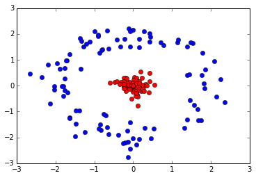
The hidden layer and output layer:
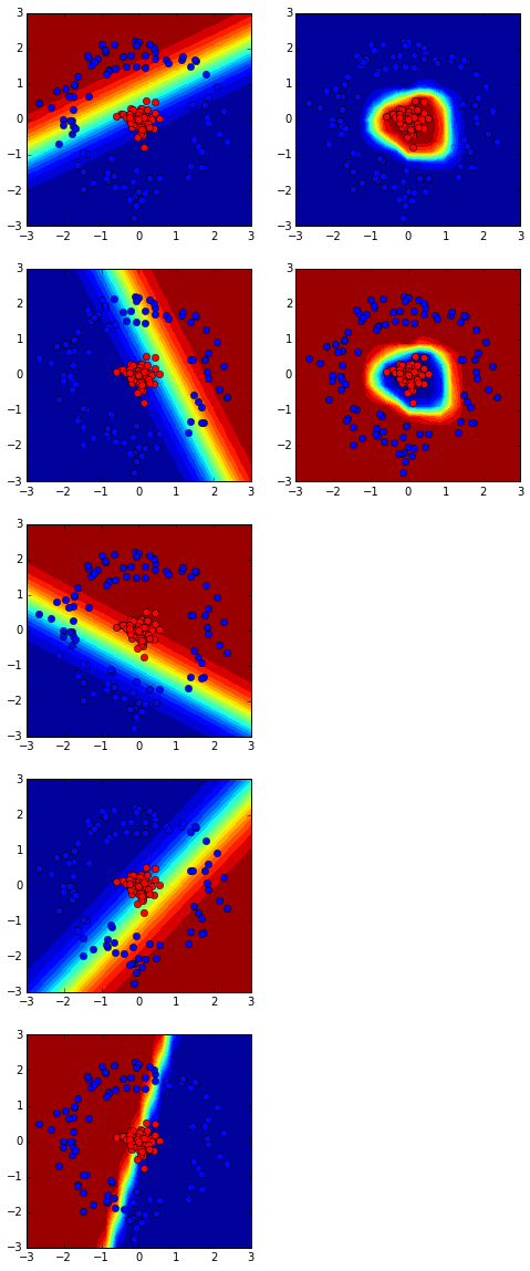
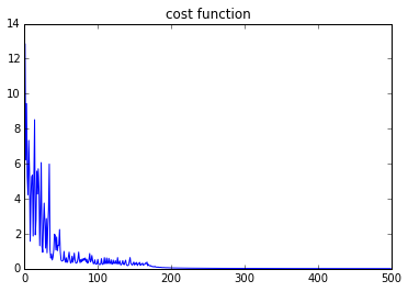
Loss function:
2.2 Tensorflow Neural Network Playground
This neural network playground is great place where you can change the settings and play with neural networks.
2.3 Scikit-learn
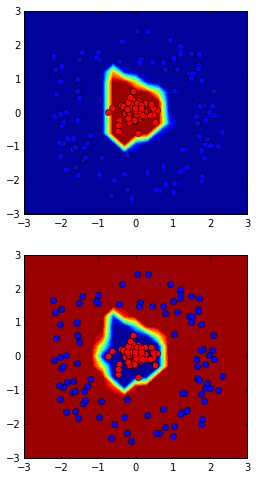
a) Tutorial of the sklearn implemented neural network
2.3.1 2D cases
nclass = 2
cstrs = ['ro','bo','go','mo','co','yo']
x,y = fxy2d_circle(m=200, nclass=nclass)

# learning
from sklearn.neural_network import MLPClassifier

clf = MLPClassifier(solver='lbfgs', alpha=1e-5, \
        hidden_layer_sizes=(5,), random_state=1, \
        activation='relu', batch_size='auto', \
        beta_1=0.9, beta_2=0.999, early_stopping=False, \
        epsilon=1e-08, learning_rate='constant', \
        learning_rate_init=0.03, max_iter=200, momentum=0.9, \
        nesterovs_momentum=True, power_t=0.5, shuffle=True, \
        tol=0.0001, validation_fraction=0.001, verbose=False, \
        warm_start=False)

clf.fit(x.T, y.T)
#clf.fit(np.append(x, x**2, axis=0).T, y.T)

# prediction
npic = 21
xx,yy = np.meshgrid(np.linspace(-3,3,npic), np.linspace(-3,3,npic))
x2 = np.append( xx.reshape(npic**2, 1), yy.reshape(npic**2, 1), axis=1)
pr = clf.predict_proba(x2)
#pr = clf.predict_proba(np.append(x2,x2**2,axis=1))


# plots
plt.figure(1, figsize=(4,8))
for irow in range(2):
    plt.subplot(2,1,irow+1)
    for i in range(nclass):
        plt.plot(x[0, y[i,:]==1], x[1, y[i,:]==1], cstrs[i])
    plt.contourf(xx,yy, pr[:,irow].reshape(npic,npic), 20)
2.3.2 High-dimension case: image recognition
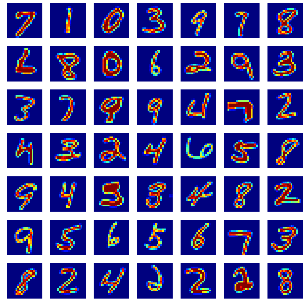
# read handwriting digits image data
data_x = np.genfromtxt('data_x.csv', delimiter=',')
data_y = np.genfromtxt('data_y.csv', delimiter=',')

# show some images from the dataset
npic = 7
plt.figure(1, figsize=(2*npic, 2*npic) )
k = np.random.choice(5000, npic*npic, replace=False)
for i in range(npic):
    for j in range(npic):
        plt.subplot(npic, npic, i*npic+j+1)
        plt.imshow(data_x[k[i*npic+j], :].reshape(20,20).T, interpolation='none', vmin=0, vmax=1)
        plt.axis('off')
plt.tight_layout()
# trainning
ntrain = 3000;  ntest = 1000

k = np.random.choice(5000, ntrain+ntest, replace=False)

clf = MLPClassifier(solver='lbfgs', alpha=1e-5, \
        hidden_layer_sizes=(25,), random_state=1, \
        activation='relu', batch_size='auto', \
        beta_1=0.9, beta_2=0.999, early_stopping=False, \
        epsilon=1e-08, learning_rate='constant', \
        learning_rate_init=0.03, max_iter=200, momentum=0.9, \
        nesterovs_momentum=True, power_t=0.5, shuffle=True, \
        tol=0.0001, validation_fraction=0.001, verbose=False, \
        warm_start=False)

clf.fit(data_x[k[0:ntrain], :], data_y[k[0:ntrain]])

# prediction
npic = 7; nrow = 5
pr = clf.predict(data_x[k[ntrain:ntrain+npic*nrow], :])

plt.figure(1, figsize=(2*npic, 2*nrow) )
for i in range(nrow):
    for j in range(npic):
        plt.subplot(nrow, npic, i*npic+j+1)
        plt.imshow(data_x[k[ntrain+i*npic+j], :].reshape(20,20).T, \
                   interpolation='none', vmin=0, vmax=1)
        plt.axis('off')
        plt.title('predict = '+format(int(pr[i*npic+j]))+'\nlabel = '+ \
                  format(int(data_y[k[ntrain+i*npic+j]])),
                  fontsize=14, loc='left')
plt.tight_layout()
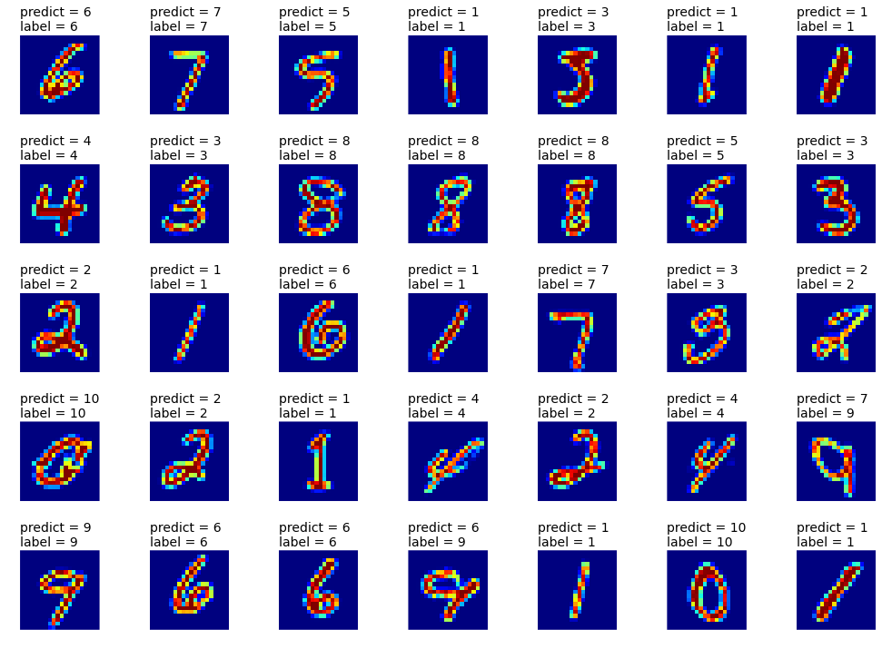
# performance on the test set
pr    = clf.predict(data_x[k[ntrain:ntrain+ntest], :]).astype(int)
label = data_y[k[ntrain:ntrain+ntest]].astype(int)

print 'Test score: ', len(label[pr==label])*1.0/ntest*100,'%'
Test score: 91.0 %
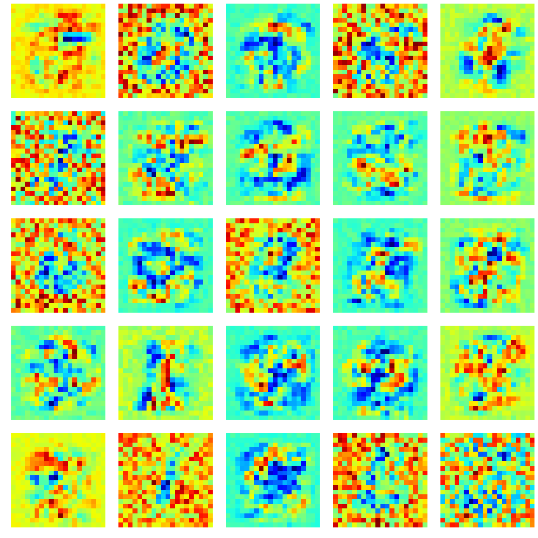
# visualize the first hidden layer weights
wts = clf.coefs_[0].T
ncol = 5; nrow = 5

plt.figure(1, figsize=(3*ncol, 3*nrow) )
for i in range(nrow):
    for j in range(ncol):
        plt.subplot(nrow, ncol, i*ncol+j+1)
        plt.imshow(wts[i*ncol+j].reshape(20,20).T, \
                   interpolation='none')
        plt.axis('off')
plt.tight_layout()
2.3.3 More examples
a) Tuning parameters
Example 1: plot the training curve
Example 2: tune the regularization
Example 3: compare different classifiers
Example 4: neural network classification on MNIST dataset
b) Autonomous game playing
https://www.youtube.com/watch?v=qv6UVOQ0F44