A short introduction of Cholesky decomposition
This blog briefly describes Cholesky decomposition and its connections with Gaussian processes and PCA.
1. Intuitive description
Consider a \(n \times p\) data matrix \(X\), which is consisted of \(p\) normalized independently and identically distributed (i.i.d) random variables with n samples. Therefore, the covariance matrix is a \(p \times p\) unit matrix:
\(\frac{1}{n}(X^T X) = I\)If there is a \(p \times p\) transform matrix \(A\) that tranforms the original independent random variables in \(X\) into a new \(n \times p\) matrix \(Y = XA\), in which some variables are linearly correlated, then the covariance matrix of \(Y\) is:
\(Q = \frac{1}{n}(Y^T Y) = \frac{1}{n}(XA)^T (XA) = \frac{1}{n}(A^T X^T X A) = A^T A\)If \(A\) can be written as an upper triangular matrix, thus \(A^T\) is a lower triangular matrix, then \(Q = A^T A\) becomes a typical Chelosky decomposition.
Therefore, given a covariance (correlation) matrix \(Q\), we can perform samplings from i.i.d random variables, by Chelosky decomposition. This is commonly used in Monte Carlo simulations.
Numpy libary provides the function linalg.cholesky() to do Chelosky decomposition:
import numpy as np

# correlated normally distributed variables
Q = np.array([[   1, 0.7, -0.5],
              [ 0.7,   1,  0.25],
              [-0.5, 0.25,    1]])

L = np.linalg.cholesky(Q)
print L

n = 200
X = np.random.normal(size=n*3).reshape(n,3)
Y = np.dot(X, L.T)
Output:
[[ 1.          0.          0.        ]
 [ 0.7         0.71414284  0.        ]
 [-0.5         0.84016805  0.21004201]]
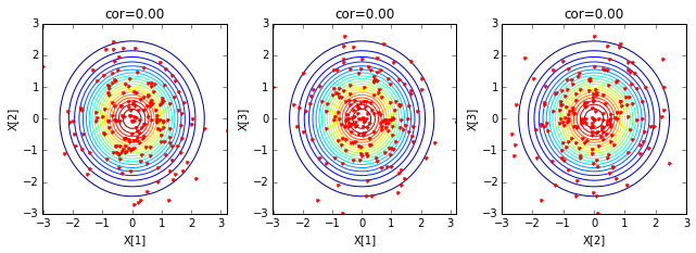
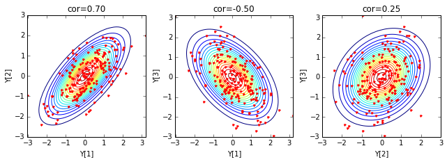
Here is an example of generating three random variables based on the covariance matrix:
import matplotlib
%matplotlib inline
import matplotlib.pyplot as plt

def mulnorm2d(x, cov):
    n = len(x)
    icov = np.linalg.inv(cov)
    dcov = np.linalg.det(cov)
    xx,yy = np.meshgrid(x,x)
    data = np.append(xx.reshape(n*n,1), yy.reshape(n*n,1), axis=1)
    pdf = np.zeros(n*n)
    for i in range(n*n):
        pdf[i] = np.exp(-0.5*np.dot(np.dot(data[i,:], icov), data[i,:]))/ \
                np.sqrt(2*np.pi*dcov)
    return pdf.reshape(n,n)


for k in ['X', 'Y']:
    if k=='X': ifig=1; data = X; cov=np.eye(3)
    if k=='Y': ifig=2; data = Y; cov=Q

    plt.figure(ifig, figsize=(9,3.3))
    for i in range(3):
        for j in range(i+1,3):
            x = np.linspace(-3,3,50)
            plt.subplot(1,3,i+j)
            plt.plot(data[:,i], data[:,j], 'r.')
            plt.contour(x,x, mulnorm2d(x, [[1, cov[i,j]],[cov[i,j], 1]] ), 21)
            plt.title('cor='+format(cov[i,j], '.2f'))
            plt.xlabel(k+'['+format(i+1)+']')
            plt.ylabel(k+'['+format(j+1)+']')
    plt.tight_layout()


2. Connection with Gaussian processes
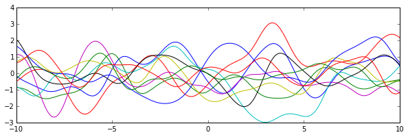
Because Gaussian processes can be seen as autoregressive models with specific kernels, which determines how the time series will look like, the Cholesky decomposition becomes very important in generating correlated multiple random variables thus the time series based on the given kernel.
def kernel(x1, x2, sigma=1.0):
    return np.exp(-((x1-x2)**2)/(2.0*sigma*sigma))

def transform(x):
    cov = np.eye(len(x))*(1+1.0e-6)
    for i in range(len(x)):
        for j in range(i+1, len(x)):
            cov[i,j] = kernel(x[i], x[j])
            cov[j,i] = cov[i,j]
    L = np.linalg.cholesky(cov)
    tmp = np.random.normal(size=len(x)).reshape(1, len(x))
    return np.dot(tmp, L.T)


t = np.linspace(-3,3,100)
x = np.linspace(-10,10,200)
plt.figure(1, figsize=(6, 3))
plt.plot(t, kernel(0,t))

plt.figure(2, figsize=(10, 3))
for k in range(10):
    y = transform(x)[0,:]
    plt.plot(x, y)
Gaussian processes kernel:

A few Gaussian processes examples:

3. Connection with eignvalue/eignvector decomposition
Consider a symmetric positive definite matrix \(A\), its Cholesky decomposition is \( A = L L^T\), and the eign-decomposition is \(A=U \Sigma U^T\), where \(U\) is an orthogonal matrix (\(U U^T = I\)) with eignvectors and \(\Sigma\) is a diagonal matrix with eignvalues.
3.1 Cholesky → Eign
Perform eign-decomposition on \(L=E \Gamma E^T\), then:
\(A = LL^T = (E \Gamma E^T) (E \Gamma E^T)^T = E \Gamma E^T E \Gamma^T E^T = E \Gamma^2 E^T\), therefore, we have \(U=E, \Sigma = \Gamma^2\).
3.2 Eign → Cholesky
Perform QR decompostion on \(U^T = QR\), where \(Q\) is an orthogonal matrix, and \(P\) is an upper triangular matrix, then:
\(A = U \Sigma U^T = (QR)^T \Sigma (QR) = R^T Q^T \Sigma Q R = R^T \Sigma R = (\Sigma^{1/2} R)^T (\Sigma^{1/2} R) \), therefore, we have \(L = (\Sigma^{1/2} R)^T\).